Building a Data Integration Cost Model That Ignores Row Counts Entirely
A three-part model prices integrations by destination, with volume costs capped.

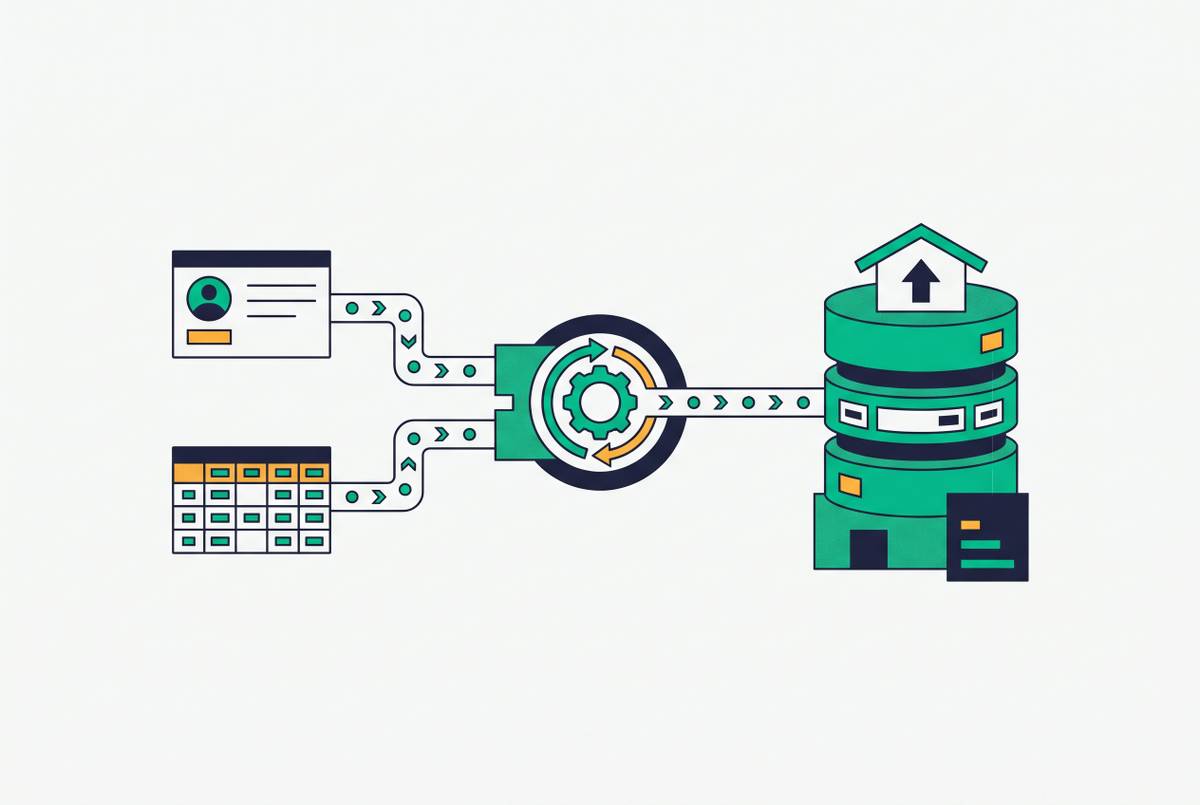
Destination-based pricing for data integration bases the bill on the systems connected. This cost model adds a per-destination charge, an adjustment for the deployment tier, and a fixed platform fee, and keeps infrastructure costs that vary with volume separate and capped. It lets product teams budget for the integrations they ship without making growth in an existing customer’s data an automatic increase in the integration bill.
Why row-count billing breaks at the moment it matters most
The month-four invoice arrives above the forecast, although the product has shipped no additional integrations. A schema change required a full-table refresh, or a nightly job updated a timestamp on every record. Under row-count billing, that activity can mark the entire table active and generate charges nobody budgeted for. Nothing new reached the customer that month. The bill increased because the source data churned.
Fivetran’s MAR model shows how billing rules can add to those costs. From January 1, 2026, deletes count as paid MAR, and history mode charges for every repeated update. Across per-row, per-task, per-connector, and flat-subscription pricing, the first three can become more expensive as a product succeeds, but per-row billing makes data growth itself a trigger. Finance must therefore forecast customer activity and infrastructure behavior to predict an integration line item, leaving unbudgeted cost cliffs to appear on invoices.
What row counts actually measure, and what cost drivers they miss
Row counts measure data churn in the source system. An orders table that updates every status field on every record can generate multiples of the MAR of a low-churn source. Yet both integrations may be just as complex and matter just as much to the business. The meter counts activity independently of whether that activity calls for more integration work.
The costs of that work follow a different pattern. They vary with the number of destination systems connected, the deployment tier required, and each destination’s compliance overhead. A single production-grade connection takes roughly 80–100 engineering hours to build, then more hours each month for maintenance, all absent from a row-count invoice. They nevertheless belong in the economic assessment because they scale with integration breadth.
For SaaS vendors embedding connectivity under their own brand, the mismatch creates another layer of exposure. The vendor absorbs charges driven by customer data churn, a rate it does not control and cannot directly infer from the integration roadmap. A useful cost model aligns spending with a shipped feature, an enterprise deal enabled, or a customer retained. For that purpose, the destination count is the appropriate unit of measure.
How to structure a destination-based cost model from first principles
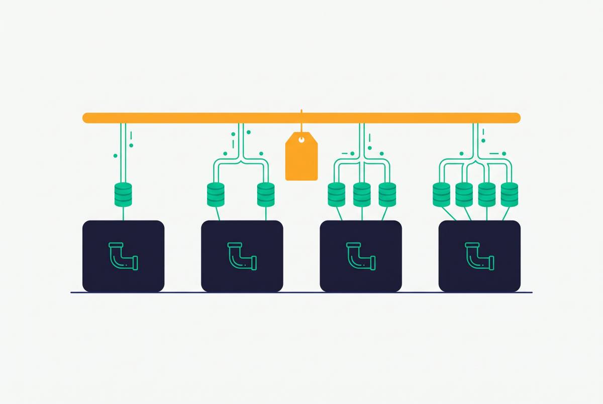
The first component is the per-destination unit cost. It prices the connection of one additional destination, regardless of the volume flowing through it. In embedded platforms, the contract may express that charge as a per-destination or named active-tenant line, making it the relevant negotiating lever during procurement. The unit needs an explicit contractual definition. A tenant-priced contract must be mapped to the product’s destinations rather than treated as interchangeable with destination pricing.
Flat subscriptions with unlimited connectors offer a different treatment of the same component. Within the subscription, the charge for each added connector falls to zero, which suits products that add many destinations quickly. That does not make every new connection costless. Engineering and maintenance work still belong in the broader assessment, but the platform fee no longer rises with each addition.
The second component is the deployment-tier multiplier. Cloud, VPC, and private or self-hosted deployment have different infrastructure and compliance costs, which belong explicitly in the model. Enterprise data residency requirements make this a procurement decision. A destination requiring VPC deployment should therefore enter the budget at that tier from the start. SOC 2 Type II certification, end-to-end encryption, and customer-managed encryption keys also belong in the capability assessment, because treating required security controls as add-ons introduces unplanned variance.
The third component is the fixed platform cost. This is the base license, SDK access, or API subscription that applies independently of destination count and data volume. It establishes the minimum recurring commitment and should be negotiated against capability tiers. Row counts, event counts, task counts, and GB transferred stay outside the integration charge. The validation test is simple and direct. If doubling the data flowing through an existing destination changes that charge, a usage meter remains in the contract.
Which data integration pricing models charge by destination instead of by row?
Flat-subscription and embedded-iPaaS pricing provide practical alternatives to row meters. The embedded and high-volume segments have moved toward these structures because unpredictable volume charges undermine the economics of products built on them. The benefit is a stable commercial unit. Under a flat subscription, the tier sets the price, with upgrades tied to capability or scale. Its strongest fit is a workload where destination variety or volume would otherwise make usage charges difficult to forecast.
The embedded iPaaS market in 2026 is organized around fixed-fee or active-tenant pricing. Active-tenant pricing connects the bill to the population served, while destination pricing connects it to the systems shipped. Neither is identical to an unlimited subscription. Their advantage is that customer data churn does not automatically determine the charge, although tenant or destination growth can still increase spending. The comparison therefore turns on what the contract counts.
Cloud, VPC, and self-hosted options price differences in compliance and infrastructure requirements. Visibility remains essential to a defensible comparison. Core-based or edition-based offers can still be opaque when professional services and other fees sit outside the quoted price. Across high-volume, high-variety, and multi-tenant workloads, the market’s convergence is toward a fixed commitment plus a destination or tenant dimension, with data volume removed from the primary integration meter.
Where row-count thinking persists and how to route around it in a cost model
Infrastructure costs can still rise with volume when rows no longer set the integration price. Change data capture, object storage egress, and compute time can all vary with workload activity. They need a separate budget boundary. For CDC, the relevant inputs are log read frequency and change velocity. A large table with little churn can be cheaper to handle than a small table with frequent changes.
Matillion bills in credits per task hour, while AWS Glue charges per unit of compute capacity used per hour. These structures price compute consumption rather than shipped destinations, and compute-sensitive costs can increase as the underlying compute becomes more expensive. The model should ring-fence or cap that exposure. Object storage sync to Amazon S3, S3-compatible stores, and similar services also introduces egress and API call costs. Those charges are typically small relative to the platform fee, but they still belong in a bounded infrastructure line.
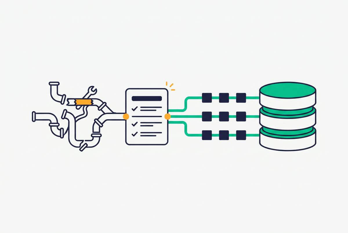
A component that doubles when customer data doubles, without new integration work, functions as a volume meter whatever its label. That volume meter needs to be identified and bounded. Passing through legitimate storage, compute, or egress costs does not require making them the organizing principle of the integration budget. Separating the two preserves an honest account of resource costs without turning each destination into an open-ended financial commitment.
How AI agent data access changes the destination count and what that means for the model
AI agents add to the systems that use synced data. Agents supporting customer service, inventory decisions, or financial positions cannot use data that is hours old when their decisions affect real-time operations. Continuous or near-continuous sync becomes part of the requirement. If each refresh is billed through a row meter, keeping data that fresh can add to the bill. A destination-based model instead associates the integration charge with the endpoint made available to the agent.
The July 2026 revision of the Model Context Protocol specification made the protocol core stateless and moved it toward request/response interactions by removing protocol-level sessions. That change cuts the infrastructure overhead of sticky-session support for hosted embedded connectors. It does not make every application stateless. The specification’s distinction is important because protocol architecture and application costs are separate questions, and statelessness alone does not define a vendor’s billing terms.
For budgeting, an MCP-accessible data endpoint is a destination. It is a connected system the product team has shipped, independent of how many rows an agent reads through it. The model needs an extension. Adding such an endpoint changes the list of destinations and may bring deployment or compliance requirements, while any rise in reads belongs within the capped infrastructure allowance.
Building the model in practice: inputs, outputs, and the questions it answers
To use the model, a product team and its finance partner need five inputs and the agreed per-destination rate on which to base the charges. The first is the current destination count, which covers the data warehouses, databases, and object storage services that now receive synced data. The second is planned destination additions with rough timing. The roadmap then drives growth in the integration budget.
The third input is the deployment tier for each destination. The need for Cloud, VPC, or private and self-hosted deployment should depend on the data residency and compliance needs of the customers it will serve. A single average can obscure that distinction. Applying the appropriate tier to each destination makes the incremental cost of an enterprise requirement visible before it enters procurement.
The fourth input is the fixed platform cost. The base license or SDK fee should be independent of destination count and negotiated against capabilities including connector breadth, sync frequency, and security certifications. The fifth input is bounded volume costs. CDC churn and storage egress enter where they are non-trivial, as capped infrastructure allowances. Keeping those allowances separate lets finance see the full cost and tell how much pays for resource use and how much pays for connectivity.
The first output is a predictable monthly baseline. It adds the fixed platform fee, the cost of current destinations at their unit rates and deployment tiers, and the separate capped infrastructure allowance. Customer data growth alone does not change the contracted integration portion. The second output is the marginal cost of shipping another destination, including its deployment requirements. Product teams can compare that figure directly with the revenue or retention value of the proposed integration.
Platforms offering embeddable SDKs, clean APIs, destination-based pricing, and no data-transfer overages make these inputs easier to collect. The way these platforms charge fits the model, so finance can work out the costs without having to work backward from a usage report. The final test belongs in the vendor conversation. A product manager should be able to answer what it costs to add one more enterprise destination with VPC deployment without calling finance. In a well-formed destination-based model, that answer is a lookup.