Snowflake Dynamic Tables for Continuous Data Delivery Pipelines
Declare the result and freshness, and Snowflake handles orchestration.

Snowflake Dynamic Tables are the most consequential shift in continuous data pipeline architecture since Streams and Tasks appeared. They let engineers specify what a transformed table should contain and how fresh it must be, then leave incremental processing, dependency resolution, and scheduling to the platform. The result is fewer objects to maintain, lower compute costs at scale, and a cleaner boundary between the data contract and the machinery that enforces it.
Why traditional Snowflake pipelines accumulate orchestration debt
The established pattern for continuous transformation in Snowflake chains three objects per pipeline layer: a Stream to track change data capture, a Task to schedule execution, and a stored procedure to run the SQL. Each object is deployed, versioned, and fails in its own way. The cost of that alignment compounds with each release because an error in any single object can break the layer silently, leaving downstream tables stale without an explicit failure signal.
Dependency ordering introduces a second source of debt. The failure mode is not a crash. It is quiet wrongness, the most expensive kind.
Scheduling adds another layer of mismatched responsibility. Cron expressions and interval configurations rarely reflect what the business actually needs, and changing them requires code changes, testing, and redeployment. The procedural model forces every layer to carry its own scheduling decision, so coordinating across layers means you compute downstream dependencies by hand.
The orchestrator itself, whether Airflow, Prefect, Dagster, or a native Task chain, demands its own compute, monitoring, and specialized expertise. When the orchestrator fails, the pipeline fails even when the data and the SQL are perfectly sound. Organizations that set out to simplify their data infrastructure often discover they have simply moved the complexity up a level, into a system they now must operate at production scale.
How Dynamic Tables replace that orchestration with a declarative contract
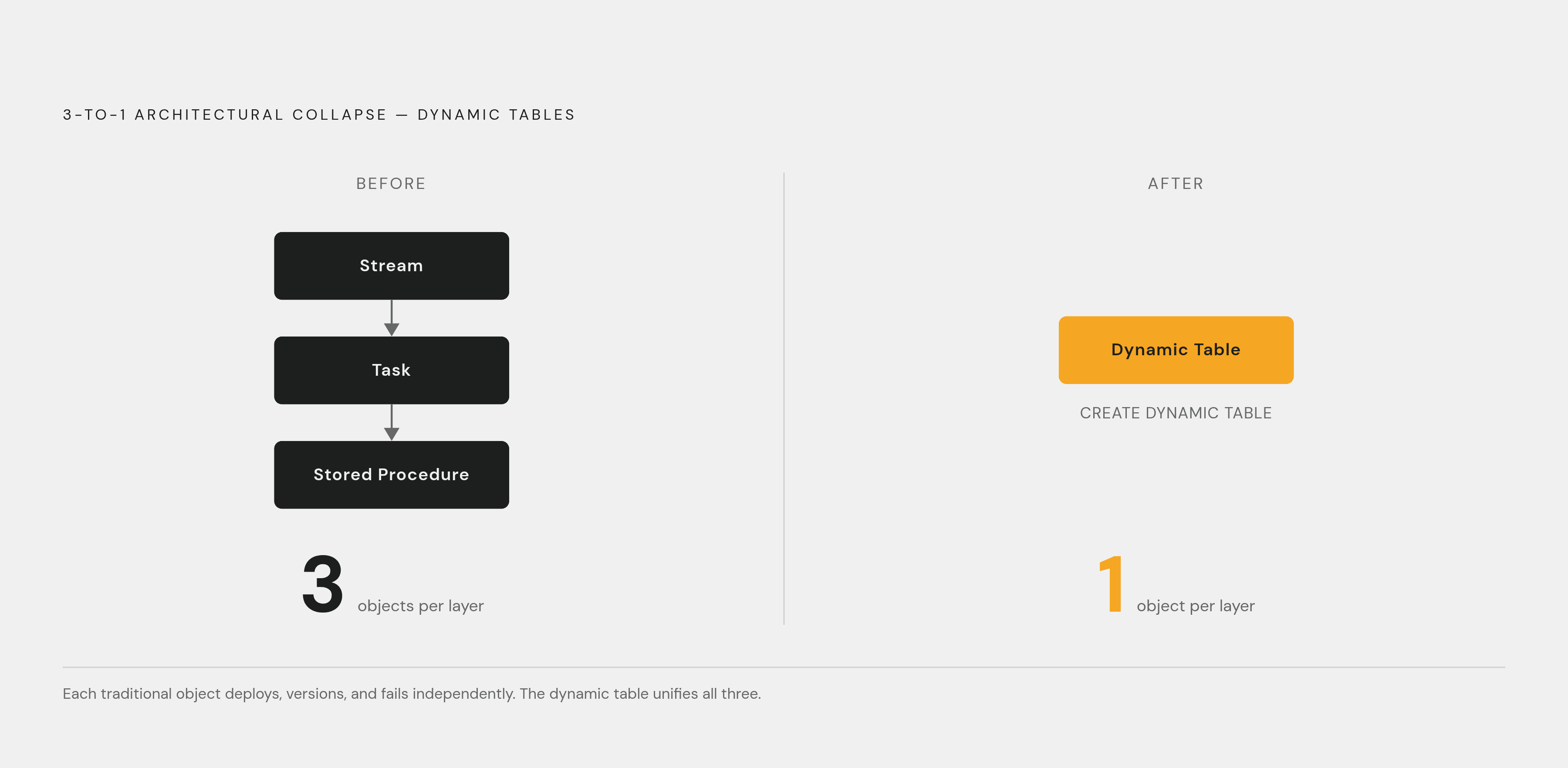
A Dynamic Table is a declarative object. The engineer writes a single SQL query defining the desired result and a freshness requirement. Snowflake infers dependencies, schedules refreshes, and processes only changed data. Where the traditional pattern requires three objects per layer, one CREATE DYNAMIC TABLE statement collapses the Stream, the Task, and the stored procedure into a single artifact. Snowflake's documented model is straightforward: define the desired state, and the platform manages incremental updates and orchestration with no manual coding and no third-party tools.
The mental model is a materialized view whose refresh frequency and incremental logic the platform controls rather than the engineer. That distinction matters because it moves the contract from procedure to declaration. The platform owns the how.
TARGET_LAG is the central configuration parameter and the clearest expression of that contract. When TARGET_LAG is set to DOWNSTREAM, the table delegates its lag decision to the Dynamic Tables consuming it, adopting the shortest target lag among all of them. That one keyword lets downstream SLAs tune an intermediate layer, not a human.
Dependency management follows the same logic. Snowflake reads the SQL definitions and auto-infers the dependency graph from the query structure itself. The graph in production is always exactly what the SQL says it is, because the SQL is the only source of truth.
How refresh modes and incremental processing work in practice
Snowflake selects among three refresh strategies, incremental, full, and adaptive, based on the query structure and upstream conditions. Understanding which strategy applies to a given table determines both its cost behavior and its latency characteristics, and the choice is not always obvious from the SQL alone. Incremental refresh processes only data that has changed since the last refresh. Some constructs, such as EXCEPT or PERCENTILE_CONT, cannot be computed incrementally and force a full refresh regardless of the target lag. If a table is small, it can cost less to recompute everything than to track changes over many tiny refresh cycles.
Adaptive refresh reached General Availability on 30 July 2026, and it changes the calculus by removing the manual decision from both directions. It runs incrementally by default but reinitializes automatically when an incremental refresh would be significantly more expensive than rebuilding from scratch, such as after an INSERT OVERWRITE or a large bulk delete. Without adaptive mode, a query incompatible with incremental refresh fails rather than silently falling back to full refresh, a deliberate design choice that surfaces construct limitations at transform time rather than masking them as performance degradation later.
What practitioners misunderstand most often is what a one-minute target lag actually means. If nothing changes, nothing refreshes. Monitoring follows the same operational surface: SHOW DYNAMIC TABLES reports status and lag, DYNAMIC_TABLE_REFRESH_HISTORY() in the Information Schema provides refresh logs, and Snowsight's visual DAG view shows failures and bottlenecks across the pipeline.
How chained Dynamic Tables form a self-managing pipeline DAG
When Dynamic Tables reference other Dynamic Tables, Snowflake constructs and manages the entire dependency graph automatically. A multi-layer pipeline from raw ingestion to serving needs no external DAG and no scheduling logic between tables. The platform derives refresh order from the SQL itself and propagates freshness requirements through the chain.
A Bronze-Silver-Gold layering pattern maps naturally onto this model. The DOWNSTREAM keyword does the propagation work: freshness requirements flow from the consuming layer back through the chain, and the platform determines the minimum refresh frequency for each intermediate table rather than requiring an engineer to specify it explicitly at every layer. A Gold table with a ten-minute lag forces its Silver and Bronze inputs to refresh at least that often, automatically.
Snowflake's DAG view in Snowsight renders the inferred dependency graph visually, giving teams native observability without standing up a third-party orchestration tool. A thirty-step transformation pipeline on Dynamic Tables has far fewer objects to track, version, and debug than the equivalent Streams-and-Tasks implementation, so it shrinks CI/CD surface area and lowers the risk of configuration drift. At this scale, the difference is not convenience. It is whether a mid-size engineering team can afford to operate the pipeline at all.
The compute cost argument for incremental refresh at scale
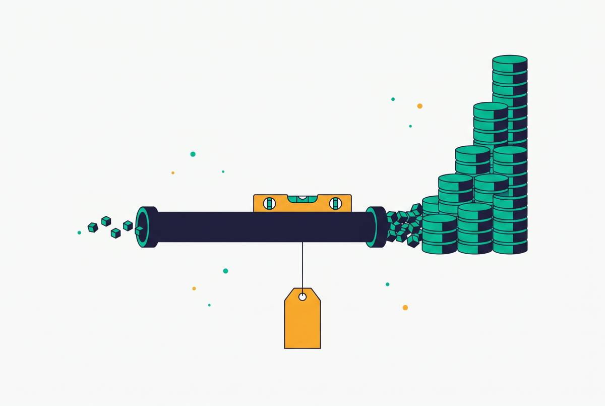
The same design choice that eliminates orchestration also reduces compute spend, and the magnitude grows with pipeline depth and data volume. Because Dynamic Tables reprocess only changed data, high-volume pipelines consume materially less compute than equivalent full-refresh Task-based pipelines. The savings compound across chained layers: each layer that filters the change set further means the next layer processes a smaller delta, not the full historical table.
The performance improvements announced at Summit 2026 quantify what that compounding looks like in production. Refresh performance improved substantially across aggregates, QUALIFY row ranking for slowly changing dimension type 1 logic, cluster-by operations, and joins. These are General Availability improvements, not previews, so teams that adopt the feature today inherit them without joining a beta program.
Dual warehouses, which reached General Availability in December 2025, separate compute pools for reads and refresh cycles. Refresh workloads no longer compete with query workloads for the same virtual warehouse, giving cost and performance predictability to both. The cost argument is strongest when these three mechanisms combine: incremental processing reduces total work, Frozen Regions eliminate redundant work on stable data, and dual warehouses ensure refresh work never degrades serving latency.
Where Dynamic Tables do not apply and Streams and Tasks still belong
Dynamic Tables replace orchestration for continuous transformation workloads, but some pipeline logic still lies outside their scope. If you name these gaps clearly, the architectural decision gets easier, not weaker. Sub-minute latency is the first hard boundary. The minimum supported TARGET_LAG is one minute, so anything faster must use Streams and Tasks. Stored procedures and external API calls are another category: Dynamic Tables are pure SQL transformation objects, so procedural logic, multi-target writes, and calls to external systems require Tasks.
Type 2 slowly changing dimension logic deserves explicit attention because it is one of the most common patterns in dimensional modeling and one of the least compatible with declarative SQL. If you build Type 2 dimensional models, keep Streams and Tasks for those layers even after adopting Dynamic Tables elsewhere in the pipeline. Complex multi-step CDC pipelines with branching write targets belong to the same category: Streams and Tasks allow conditional logic across multiple destination tables, which a declarative single-target transform cannot express.
These are not weaknesses of the feature. They are a clear division of responsibility that makes the choice of tool simpler: if the logic fits a declarative SQL transform with a one-minute or longer lag, Dynamic Tables are the answer. If it does not, it never will, and investing in Streams and Tasks for that layer is the correct call.
How Dynamic Tables and dbt divide transformation responsibility in a modern pipeline
The most practically consequential design question for teams already using dbt is where to draw the boundary between dbt models and Dynamic Tables. The emerging 2026 production pattern puts Dynamic Tables in the Silver layer for continuous freshness instead of simpler dbt models, but it keeps dbt for Gold-layer business logic where test coverage and documentation are critical outputs. Teams do not have to choose one tool over the other at the project level. The boundary is set at the model level based on freshness requirements and governance needs.
The answer to that objection is not that tests do not matter. Dynamic Tables fit the first case. dbt fits the second. The tools complement rather than substitute for each other, and the boundary between them is where the strongest architecture keeps it: at the layer where the primary SLA changes.
What changed at Summit 2026 and in the late 2024–2025 release cycle
The capabilities described throughout this piece reflect a mature and actively evolving platform, not a preview-stage experiment. The release arc from late 2024 through mid-2026 shows a consistent through-line: each release addresses a specific class of pipeline that previously required external tooling or manual intervention. Summit 2026 delivered the headline performance improvements: substantially faster refresh across aggregates, QUALIFY row ranking, cluster-by operations, and joins, as General Availability. The feature now runs incrementally by default and reinitializes automatically when an upstream change makes incremental refresh more expensive than a full rebuild.
The 2025 releases filled structural gaps. CREATE OR ALTER DYNAMIC TABLE reached Preview in September 2025, allowing live schema alteration without tearing down and rebuilding the pipeline. With the UNION change, pipelines that use that operator no longer have to take a full refresh. Dual warehouses provide separate compute pools for reads and refresh, eliminating the resource contention that could make refresh workloads visible to end users.
AI agent data access through Dynamic Tables and what it requires architecturally
Dynamic Tables are a natural data layer for AI agents because freshness is guaranteed by the platform rather than by the agent's caller. AI and ML systems require continuously fresh data: feature stores, real-time scoring models, and AI-powered product experiences break down when the underlying data is stale. Dynamic Tables give you that freshness with no separate serving layer between the warehouse and the model. Snowflake's Dynamic Tables feature page lists a certified solution, "Build Autonomous Pipelines for AI," dated May 26, 2026, as a current resource, and Cortex AI Functions now run directly within the Dynamic Table transformation layer rather than as a post-processing step.
The architectural shift is most visible in security. Agent Identity, announced at Summit 2026, gives autonomous agents cryptographically verified identities when they access Snowflake data, so zero-trust security now extends to the agents consuming pipeline output, not only the humans and services that accessed it before. The Cortex Agent SDK, in Public Preview as of October 2026 for Python and TypeScript, supports applications running Cortex Agents and Cortex Code that maintain conversations, observe durable turns, and reconnect to long-running work. Dynamic Tables become the data substrate these agents query, which means the freshness and security guarantees must be owned by the table definition, not by the calling application.
What continuous delivery pipelines mean for SaaS products that sync to customer data warehouses
For SaaS products that deliver data to customers' own warehouses, the declarative freshness model of Dynamic Tables defines what the product is responsible for and what the customer's environment handles. When a SaaS vendor writes data into a customer's Snowflake environment, the vendor controls the transformation and freshness guarantees. The customer retains full control over their environment, query patterns, and downstream consumers. That separation is valuable because it means the vendor can ship a freshness SLA as a product feature rather than as an operational promise backed by manual monitoring.
How to decide where Dynamic Tables belong in a production pipeline architecture
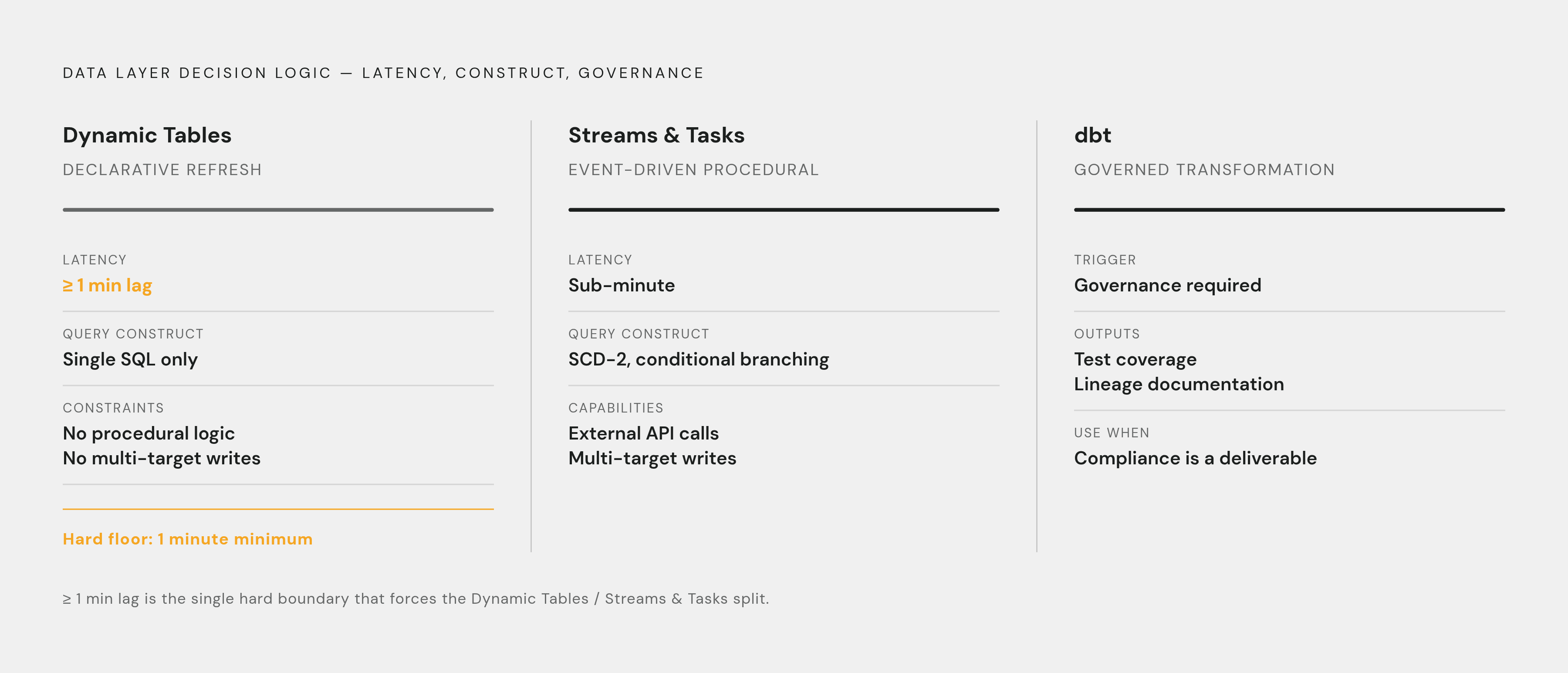
The decision of whether to use Dynamic Tables, Streams and Tasks, or dbt is not a global one. It is made at the layer level based on three criteria: latency requirement, query construct compatibility, and governance output. Dynamic Tables are the right choice when the transformation is expressible in a single SQL query, the acceptable lag is one minute or more, and the primary SLA is freshness rather than audit documentation. Streams and Tasks are required when latency must be sub-minute, the logic requires stored procedures or external API calls, or the pattern involves writing to multiple targets conditionally, including Type 2 slowly changing dimension history maintenance. dbt, potentially with Dynamic Table materialization, belongs where the pipeline serves compliance-critical outputs, test coverage and lineage documentation are required deliverables, or the Gold layer business logic benefits from dbt's package ecosystem and peer review workflows.
For teams migrating from a Streams-and-Tasks architecture, the practical starting point is identifying the transformation layers with the highest orchestration overhead and the clearest SQL-expressible logic. SCD-2 layers and sub-minute CDC layers stay on Streams and Tasks. Adaptive Refresh, generally available as of July 30, 2026, removes one of the last manual judgment calls: teams no longer need to decide when to force a full refresh after a bulk load because the platform handles it.
The declarative model's core value is not performance or cost, though you get both. It moves the engineer's attention from whether the pipeline is running correctly to whether the data is correct. That is a different kind of work, the kind that was the point all along.